How to acknowledge data from the RAPID-MOCHA project:
Data from RAPID-MOCHA monitoring project are made freely available to the public. The project scientists would appreciate it if you added the following acknowledgment to any publications that use this data:
"Data from the RAPID-MOCHA program are funded by the U.S. National Science Foundation and U.K. Natural Environment Research Council and are freely available at www.rapid.ac.uk/rapidmoc and mocha.earth.miami.edu/mocha."
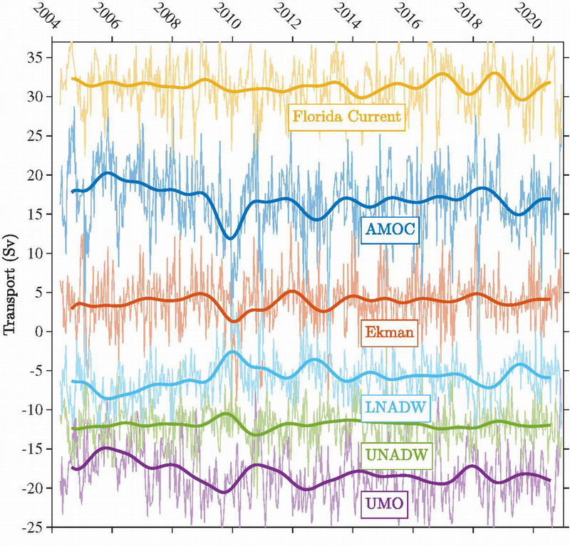 |
The AMOC time series and components
Time series of Florida Current transport (yellow), Ekman transport (red), upper mid-ocean transport (purple) and overturning transport (dark blue) for the available record from 2004 to 2020. Also shown are the basinwide transports in the upper and lower NADW layers (UNADW: 1100-3000 m; LNADW: 3000-5000 m; green and light blue lines, respectively). The high-frequency data represent 10-day averages while the superimposed curves are 18-month lowpass filtered data after removal of each series' climatological seasonal cycle
Adapted from Johns et al. (2023) [in press].
|
|
|
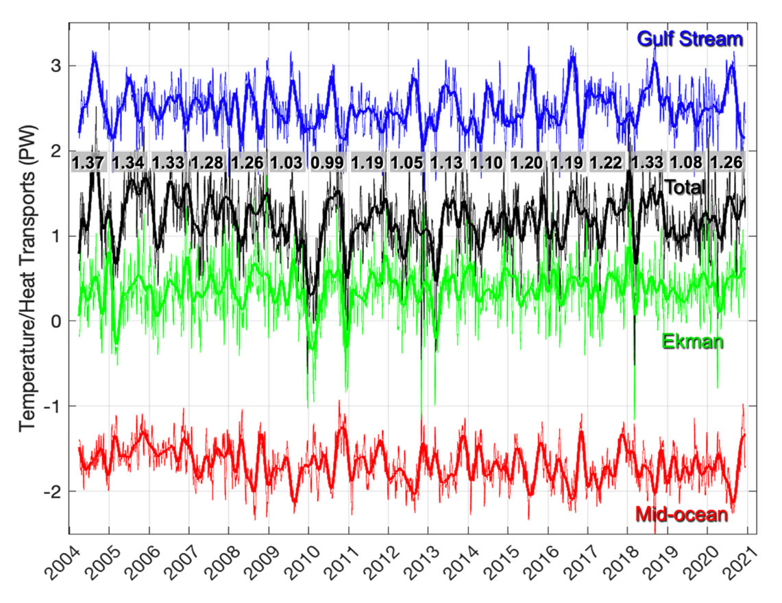
The MHT time series with main components and annual averages
Time series of net meridional heat transport (black), and temperature transports (relative to 0°C) of the Gulf Stream (blue), Ekman layer (green), and Mid-ocean region (red). Thin lines are 10-day averages and thick lines are 90-day lowpass filtered results. Annual averages of the net heat transport are shown in gray boxes.
Adapted from Johns et al. (2023) [in press].
|
|
|
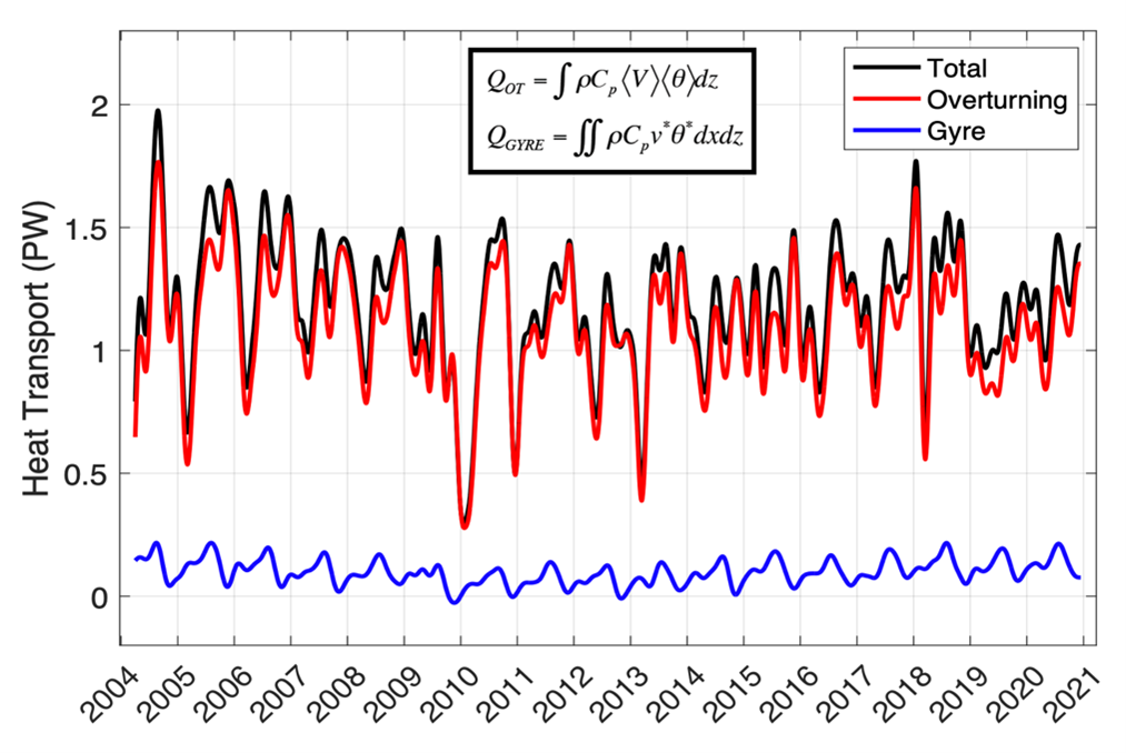
The overturning and gyre heat transports
Heat transport decomposition into an "overturning" component (QOT, derived from the zonally averaged velocity and temperature in depth coordinates, red curve), and a "gyre" component (QGYRE, derived from velocity and temperature anomalies with respect to the zonal mean, also computed in depth coordinates, blue curve). Total heat transport is shown in black; all time series are 90-day lowpass filtered.
Adapted from Johns et al. (2023) [in press].
|
Looking for downloadable data? Visit our Data tab!